Introduction

The paper “FMMI: Flow Matching Mutual Information Estimation” (Butakov et al. 2025) proposes a new way to estimate MI by learning a continuous normalizing flow that transports the product of marginals $P_X \otimes P_Y$ into the joint distribution $P_{X,Y}$, and then reading MI off from the divergence of the learned velocity field.

In this post, we’ll walk through:

1. The core idea: MI as a KL divergence and as a difference of entropies
2. Continuous flows and the identity $\displaystyle \frac{d}{dt} \log p_t(x_t) = -\operatorname{div} v(x_t,t)$
3. A key lemma: entropy difference as an expectation of divergence
4. How Flow Matching learns the velocity field from samples
5. How all of this specializes to a mutual information estimator (jFMMI)
6. The Monte-Carlo / Hutchinson’s trick implementation

1. Mutual Information and the product of marginals

Let $X$ and $Y$ be random vectors with joint distribution $P_{X,Y}$ and marginals $P_X$, $P_Y$. The mutual information is

where $P_X \otimes P_Y$ is the product measure (the joint distribution you’d get if $X$ and $Y$ were independent).

If densities exist, we also have the familiar entropy identities

with differential entropy $h(X) = -\mathbb{E}[\log p_X(X)]$.

The FMMI paper will express entropy differences via flow matching, and then plug those into these identities to get MI.

2. Continuous flows and divergence

Continuous normalizing flows describe a time-dependent random variable $X_t$ via an ODE

where $v(x,t)$ is a velocity field. Let $p_t$ be the density of $X_t$. Under mild regularity, continuous flows satisfy the classic identity

This is equivalent to the continuity equation

and can be seen as the continuous-time version of the change-of-variables formula.

Integrating (1) along the trajectory $X_t$ from $t=0$ to $t=1$ gives

Taking expectations will connect divergence to entropy; that’s the next step.

3. Entropy difference = expectation of divergence (Lemma 4.1)

Define differential entropy

Differentiate w.r.t. time using (1):

Integrate from $t=0$ to $t=1$:

If we now draw $T \sim \mathrm{Uniform}[0,1]$ and consider the joint distribution of $(X_T, T)$, this integral can be written as a single expectation:

4. Learning the velocity with Flow Matching

Of course, in practice we don’t know the true velocity $v$. We only have samples from $P_0$ and $P_1$.

Flow Matching (Lipman et al.) gives a way to learn $v_\theta(x,t)$ from samples alone, by turning the CNF problem into a regression problem on velocities.

The trick is:

• Pick a simple conditional path between two endpoints $x_0 \sim P_0$ and $x_1 \sim P_1$, e.g. linear interpolation $$X_t = (1-t) X_0 + t X_1$$
• This path has a known conditional velocity $$v(x_t,t \mid x_1) = x_1 - x_t$$

Flow Matching says: instead of integrating the ODE during training, just regress a neural network $v_\theta(x,t)$ on these conditional velocities. Concretely, the FM objective is:

When this regression succeeds, the marginal flow induced by $v_\theta$ transports $P_0$ to $P_1$ in the same way the “true” flow would.

This is what the paper calls FMDoE (Flow Matching Difference of Entropy): first learn $v_\theta$ by FM, then use (2) to estimate entropy differences via divergence.

5. From entropy differences to mutual information

Now we connect this to mutual information.

Recall one of the entropy forms of MI:

The idea in FMMI is:

1. Build flows between carefully chosen distributions, so that entropy differences recover MI.
2. Use FMDoE to estimate those entropy differences via divergence expectations.

jFMMI: joint-based estimator

The simplest variant, jFMMI, chooses:

• $P_0 = P_X \otimes P_Y$: product of marginals
• $P_1 = P_{X,Y}$: joint distribution

Let $Z=(X,Y)$. Under $P_0$, $Z_0 \sim P_X \otimes P_Y$, while under $P_1, Z_1 \sim P_{X,Y}$. Then:

• Entropy at (t=0): $$h(Z_0) = h(X) + h(Y)$$ since $X$ and $Y$ are independent under $P_X \otimes P_Y$.
• Entropy at (t=1): $$h(Z_1) = h(X,Y)$$

So the entropy difference is

Combine this with the DoE identity (2):

where $v$ is any velocity field whose flow maps $P_X \otimes P_Y$ into $P_{X,Y}$. Therefore,

This is the key theoretical identity behind jFMMI: mutual information is the negative divergence expectation of any flow that transports the product of marginals into the joint.

In practice we don’t know $v$, so we plug in the learned $v_\theta$:

That’s jFMMI.

6. Estimating divergence in practice: Hutchinson’s trick

To use (5), we need $\operatorname{div} v_\theta(z,t)$, without computing a full Jacobian.

Let

Hutchinson’s estimator says: if $\varepsilon \sim \mathcal{N}(0,I_d)$, then

So an unbiased estimate is:

1. Sample $\varepsilon \in \mathbb{R}^d$,
2. Compute the scalar $$s = v_\theta(z,t) \cdot \varepsilon$$
3. Backpropagate $\nabla_z s = J^\top \varepsilon$,
4. Form $$\widehat{\operatorname{div} v_\theta}(z,t) = \varepsilon^\top J \varepsilon = \sum_i \varepsilon_i (\nabla_z s)_i$$

This requires only one backward pass per point, instead of $d$ passes.

7. Monte-Carlo implementation of jFMMI

Putting everything together, FMMI implements (5) via simple Monte-Carlo:

1. Sample a batch of pairs $(z_0,z_1)$ where
   • $z_1 \sim P_{X,Y}$ (true joint),
   • $z_0 \sim P_X \otimes P_Y$ (shuffle Y independently to break dependence).
2. Sample $t \sim \mathrm{Uniform}[0,1]$.
3. Build the interpolated points $$z_t = (1-t) z_0 + t z_1$$
4. Evaluate the learned velocity field $v_\theta(z_t,t)$.
5. Estimate the divergence $\widehat{\operatorname{div} v_\theta}(z_t,t)$ via Hutchinson.
6. Each sample gives a stochastic MI contribution $$\hat I_i = -\widehat{\operatorname{div} v_\theta}(z_t^{(i)}, t^{(i)})$$
7. Average over many samples: $$\widehat{I(X;Y)} = \frac{1}{N}\sum_{i=1}^N \hat I_i$$

8. Why this is interesting

Compared to classic discriminative MI estimators, FMMI:

• avoids large batch / negative sampling issues,
• does not require directly estimating density ratios,
• scales better to high MI regimes (where joint and product distributions are very far apart),
• and leverages the modern, well-understood machinery of flow matching.

Conceptually, it reframes MI estimation as:

Learn a path that morphs independence into the true joint, and read MI as the total log-volume change along the way.

Once you see MI as entropy difference, and entropy difference as expected divergence of a flow, the whole construction becomes very natural.

Experiments

To validate the jFMMI estimator introduced in the paper, we designed a controlled numerical experiment where the true mutual information (MI) is known analytically. This allows us to measure estimation accuracy, bias, and convergence of the proposed method.

Synthetic Data Setup

We consider a simple bivariate Gaussian model:

With this construction, the mutual information has a closed-form:

We set $\rho = 0.9$, giving a ground-truth MI of:

We generate 30,000 samples from the joint distribution $P_{X,Y}$. To obtain samples from the product of marginals $P_X \otimes P_Y$, we shuffle the $Y$ values independently from $X$. This gives endpoints $(Z_0, Z_1)$ for flow matching.

Flow Matching and Velocity Network

We train a neural velocity field $v_\theta(z,t)$ with 512 hidden units and Tanh activations to match the true conditional velocity along the linear path:

The Flow Matching loss is:

The model is trained for 5,000 gradient steps with AdamW and cosine annealing.

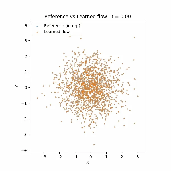
Although the FM loss exhibits mild oscillation, the flow nonetheless converges well: the learned transport visually matches the ground-truth Gaussian interpolation when animated.

Mutual Information Estimation

After training, we estimate MI using the jFMMI identity:

with divergence estimated via Hutchinson’s estimator:

We draw 50,000 Monte-Carlo samples $(Z_t,t)$ to approximate the expectation.

Results

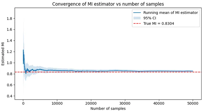
The estimator converges towards the true MI:

• True MI: 0.8304
• Estimated MI (jFMMI): ≈ close to the true value
• Standard error: small (scales as $1/\sqrt{N}$)

The curve $N \mapsto \hat I_N$ shows fast convergence but a small positive bias, expected due to imperfect learning of the velocity field. Increasing network depth significantly reduces this bias, confirming the role of expressivity.

Flow Visualization

We additionally animate the learned flow and the ground-truth flow simultaneously. The trajectories of particles under both flows almost perfectly overlap, demonstrating that the learned $v_\theta$ captures the correct transport from $P_X\otimes P_Y$ to $P_{X,Y}$.

This visual inspection confirms that Flow Matching learned the intended probability path, validating the theoretical assumptions behind jFMMI.