The Muon optimizer (MomentUm Orthogonalized by Newton–Schulz) has rapidly evolved since its introduction in late 2024. In this article, we retrace the history of Muon from the original idea to its latest adaptations. Muon’s development showcases how principled mathematical ideas, like orthogonalization of updates and adaptive norms, translate into state-of-the-art training efficiency for neural networks.
The Birth of Muon (October 2024)
Muon was first introduced by Keller Jordan et al. in October 2024 via a detailed blog post as an optimizer specialized for weight matrices in neural network hidden layers. The key idea was to treat a weight matrix (and its gradient ) not as a flattened vector (as in standard optimizers), but as a matrix with structured geometry. Empirically, it was observed that gradient updates for linear layers (e.g. in Transformers) often have extremely high condition number, in other words, the update matrix is “almost” low-rank, with a few dominant singular directions and very small components in other directions.
This imbalance suggests that learning could be improved by equalizing the update across directions. Muon addresses this by orthogonalizing the update matrix, amplifying those rare directions in the gradient that would otherwise be overshadowed by the top singular directions.
Mathematically, Muon builds on the Nesterov accelerated gradient (NAG) update. Let be the current gradient of the loss with respect to weight matrix , and let be the momentum coefficient (e.g. 0.95). Define a momentum accumulator as an exponential moving average of gradients:
with . One then computes a lookahead update matrix (sometimes called the Nesterov “approximated gradient”):
Here is essentially the momentum-corrected gradient update at time . Muon’s distinctive step is to replace with an orthogonalized version before applying it to the weights. Specifically, Muon seeks the closest matrix to that is semi-orthogonal (having orthonormal columns or rows):
where is the Frobenius norm. In simple terms, is the matrix closest to that has orthonormal vectors (either column-wise or row-wise depending on the shape). It can be shown that the solution is given by the singular value decomposition (SVD) of . Let,
be the SVD of , where and are orthogonal matrices containing the left and right singular vectors, and is the diagonal matrix of singular values. The optimal orthogonal approximation is obtained by replacing all singular values with 1, yielding
which indeed satisfies (for a tall ) or (for a wide ), and is the closest such matrix to in Frobenius norm.
Performing an exact SVD for every update is computationally expensive. Muon circumvents this by using a Newton–Schulz iterative method to approximate efficiently. The Newton–Schulz iteration is an iterative polynomial that converges to the matrix sign function (which would map to in the SVD). Muon’s implementation normalizes the update matrix first (since the orthogonal direction is scale-invariant): let
so that all singular values of lie in . Then it iteratively applies a fixed cubic polynomial on the matrix:
for (with steps in the original implementation). The coefficients are tuned constants (, , ) chosen so that quickly drives singular values toward 1 when iterated, even in low precision arithmetic. Intuitively, this polynomial is an odd function (only odd powers of ), which ensures that preserves the SVD eigenspaces of . Repeated iteration of pushes each singular value closer to 1 (the fixed-point of the sign function). After iterations, we obtain . The weight update is then applied as:
with the learning rate. In effect, Muon takes the momentum step and whitens it before updating the weights: scaling up the small singular directions and scaling down the largest ones.
The Newton–Schulz approach is extremely fast: only a fixed number of matrix multiplications (5 in practice) per update, adding under 1% computational overhead to training. The coefficients were graphically tuned to maximize convergence speed while keeping the intermediate matrix values numerically stable (ensuring singular values stay roughly in the range through the iterations even if starting in ), a critical consideration for bfloat16 precision.
Notably, Muon’s update is closely related to Shampoo, Gupta et al. 2018: if one were to remove momentum and use the raw gradient instead, an idealized Shampoo update would compute , which algebraically simplifies to (since for ).
In other words, Shampoo without accumulated statistics would produce the same orthogonalized direction as Muon. Muon’s novelty was to apply this orthogonalization on each momentum update, integrating seamlessly with SGD-momentum.
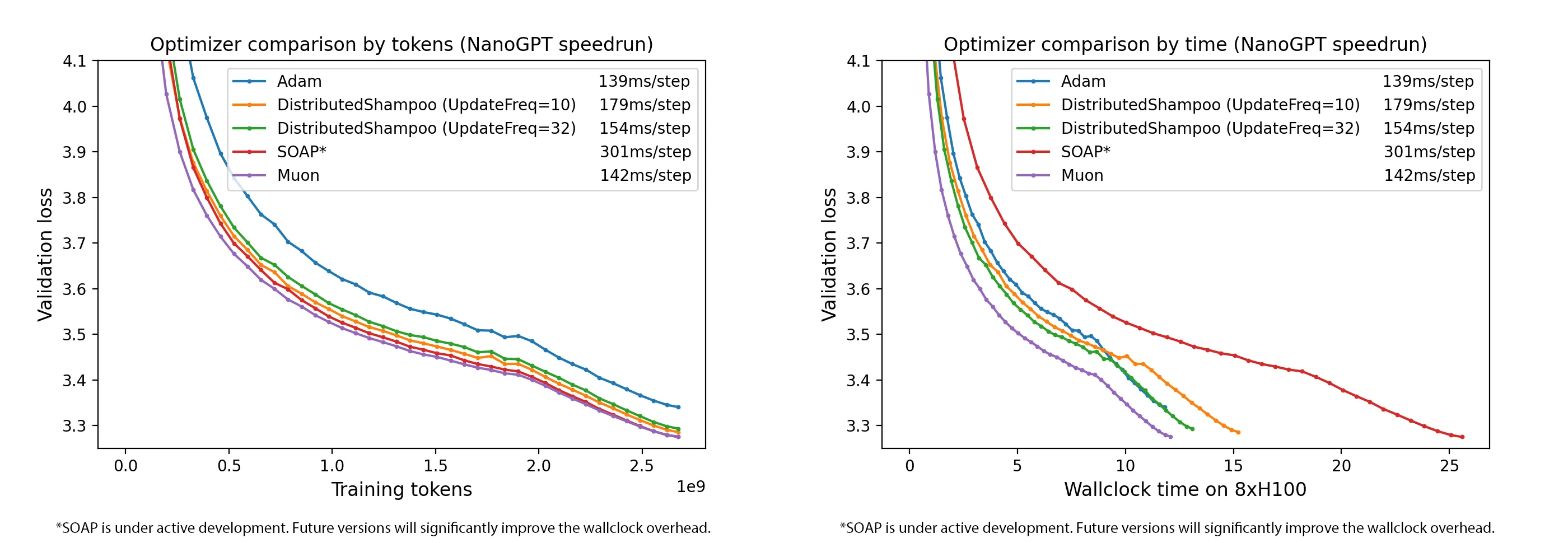
Results and impact: The introduction of Muon led to remarkable empirical gains. By orthogonalizing updates, Muon achieved faster training on multiple benchmarks. For example, using Muon set new speed records in late 2024, including training a CIFAR-10 classifier to 94% accuracy ~21% faster (reducing time from 3.3 to 2.6 seconds on A100) and improving the NanoGPT (FineWeb) language model training loss at a given compute budget by a factor of 1.35× (about 35% faster convergence). Muon continued to show benefits at scale, improving sample efficiency in models up to 1.5B parameters.
Scaling Muon for LLMs: Weight Decay and RMS Alignment (February 2025)
As Muon gained attention, researchers began adapting it for large-scale models, including billion-parameter language models. In February 2025, Moonshot AI released a technical report addressing how to make Muon effective for large language model (LLM) training, Liu et al . 2025. Two key modifications were introduced: weight decay integration (like AdamW) and a rescaling of updates to fix shape-dependent quirks.
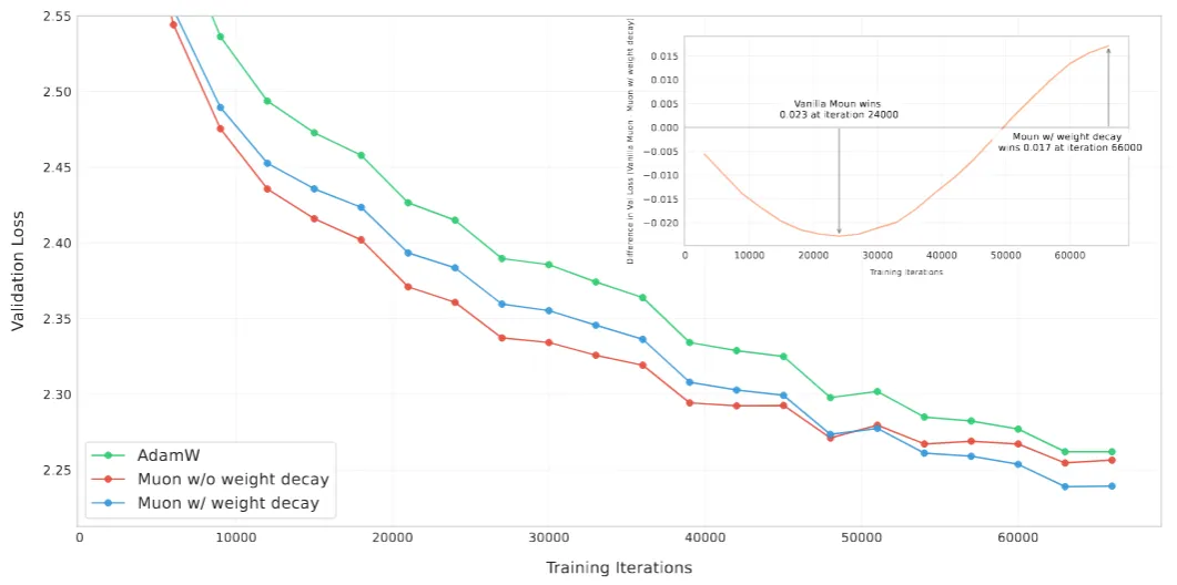
Weight Decay: Classic AdamW optimizer includes a weight decay term (-regularization) decoupled from the gradient update. The Moonshot team found that adding a similar weight decay term to Muon was important for stable and generalizable training of big models. They modified the update rule to:
where is the Muon update matrix (orthogonalized momentum, denoted above) and is the weight decay coefficient. In their experiments a was used. This decoupled weight decay helped Muon match the generalization performance of AdamW on large-scale tasks while still benefiting from faster convergence.
RMS Alignment (Update Rescaling): An interesting observation was that Muon’s update magnitude depends on the shape of the weight matrix. In Muon, an orthogonalized update has Frobenius norm that is inversely proportional to the square root of the larger dimension of . In fact, for an weight matrix, one can show the expected root-mean-square (RMS) of an ideal Muon update is .
This means layers with very large width or height would get systematically smaller updates (in RMS terms) than layers with smaller dimensions, when using the same learning rate. By contrast, optimizers like AdamW tend to produce updates with more uniform RMS magnitude across layers (often in the range 0.2–0.4 in the units of weight initializations). To balance the update magnitudes across different layer shapes, Moonshot AI introduced a scaling factor. They chose to scale Muon updates such that their RMS matches a reference value around 0.2 (matching a typical AdamW update RMS). Concretely, if is the orthogonalized momentum at step , they compute:
and then rescale the update by a factor (since ). The update rule becomes:
which for convenience can be implemented as
since for orthogonal . This adjustment ensures every layer (regardless of its shape) receives updates of comparable RMS scale, making a single learning rate work well across the whole model without per-layer tuning.
With these changes—orthogonalized momentum + weight decay + RMS-aligned scaling—Muon became highly effective for large Transformers. The team demonstrated scaling law improvements: in their experiments, a given loss could be reached with roughly half the compute compared to AdamW.
For example, fits to loss-vs-compute curves showed Muon achieving a certain loss with 52% of the FLOPs required by AdamW, essentially a 2× training efficiency gain. Moreover, analyzing the distribution of singular values of updates, they found Muon’s updates had significantly higher entropy (i.e. a flatter singular value spectrum) than AdamW, indicating Muon utilizes a broader set of directions in the weight space during training (consistent with the orthogonalization idea). In practice, Moonshot’s 16B-parameter Moonlight-MoE model (a mixture-of-experts Transformer) trained with Muon achieved notable performance gains: for instance, on the MMLU benchmark it scored ~70.0% accuracy versus 65.6% for a comparable AdamW-trained baseline.
These results cemented Muon as a viable successor to AdamW for large-scale training. The team also introduced a distributed implementation (using ZeRO-1 sharded optimizer state) that reduced memory overhead by roughly 2×, enabling Muon to be applied to multi-billion-parameter models without memory bottlenecks.
Deriving Muon: RMS Norms, Duality, and Width-Independence (March 2025)
In March 2025, Jeremy Bernstein published a blog post titled “Deriving Muon”, providing a theoretical derivation of the Muon update from first principles. This work framed Muon as the solution to an optimization problem under a particular norm constraint, shedding light on why Muon yields width-independent training dynamics (i.e. stable behavior as layer widths increase).
The derivation begins by defining an appropriate norm for the linear layer. For a weight matrix (with outputs, inputs):
-
The RMS norm of a vector is . This is just the Euclidean norm normalized by the square root of the dimension, so that a “dense” vector of roughly unit-sized components has .
-
The RMS→RMS operator norm of a matrix is defined as the maximum factor by which can stretch a vector’s RMS norm. Formally, . It turns out that this is just a scaled version of the spectral norm of . In fact where is the largest singular value of . The factor accounts for the normalization of input and output by and respectively.
Bernstein then considers one step of gradient descent under this RMS norm constraint. Suppose we have current weights and loss gradient of the same shape. We ask: what is the best update that minimizes the linearized loss, subject to a limit on the RMS→RMS norm of the update? This can be written as the constrained optimization problem:
where is a small step size controlling the allowed change in output RMS. Because is the first-order loss increase (the dot product of gradient and update), minimizing it means we want to be in the steepest descent direction of the loss. The constraint, however, prevents from being too large in the RMS→RMS sense (thereby controlling how much the outputs can change in RMS norm).
Using the SVD of the gradient, , one can solve this constrained problem analytically (via the method of Lagrange multipliers or simply by intuition of aligning with the gradient). The solution is:
which is remarkably the orthogonalized gradient (up to the same factor we saw earlier). In words, the optimal constrained update keeps the left and right singular vectors of the gradient, but sets all singular values equal (and scaled to meet the norm bound). This is exactly Muon’s update direction: . The factor adjusts for the norm definition and ensures the update saturates the constraint .
This derivation provides a principled justification for Muon: it is performing (approximate) steepest descent in the RMS norm, which has the effect of balancing updates across neurons and is linked to width-independent learning rates. In fact, one corollary is that if you scale up a layer’s width (increase or ) and initialize appropriately, Muon’s effective step size on the outputs remains the same. This phenomenon, sometimes called μP (maximal update parametrization) style width invariance, emerges naturally from Muon’s norm choice.
Finally, Bernstein addressed the practicality: solving the constrained step exactly would require SVD (expensive), so he recapitulated the idea of using a Newton–Schulz iteration to achieve the orthogonalization efficiently. He noted that an odd polynomial like:
applied iteratively, will push a matrix’s singular values toward 1 (this is a simple case of the Newton-Schulz update). Higher-order tuned polynomials (like the 5-step one used in Muon) can accelerate this convergence. Thus, the combination of dualizing the gradient under RMS norm and fast Newton–Schulz orthogonalization yields the Muon algorithm. This theoretical lens helped validate Muon’s design and provided insights into how it achieves faster convergence and robustness to width. It also fit into a broader research program of developing “modular” optimizers tailored to specific layer types.
Convergence Analysis: Faster Rates Under Low-Rank Hessians (May 2025)
As interest in Muon grew, researchers investigated its convergence properties. In May 2025, a theoretical analysis was released by Newhouse et al. providing convergence guarantees for Muon in certain settings, and comparing these to standard gradient descent. The analysis focused on scenarios where the loss function’s Hessians are approximately low-rank or have a block structure – reflecting the intuition that Muon excels when gradients lie in a low-dimensional subspace.
Under standard assumptions of smoothness, they considered two Lipschitz constants: a Frobenius smoothness constant (such that for all weights) and a possibly smaller spectral smoothness constant (such that , where is nuclear norm and is spectral norm). Intuitively, if the Hessian at any point has rank lower than full, or its eigen-spectrum decays (so its largest eigenvalue is much larger than the sum of eigenvalues). In such cases, Muon’s updates (which effectively operate in the top eigenspace of gradients) can exploit this structure.
The results showed that Muon converges in fewer iterations than gradient descent when the gradient covariance or Hessian is low-rank. For example, in a non-convex stochastic setting, to reach an -approximate nuclear stationary point (where the gradient’s nuclear norm is small), Muon was shown to require iterations (where is an initial optimality gap), whereas standard gradient descent requires iterations, with the effective rank of the Hessian. Since can be much smaller than in the presence of low-rank structure, this indicates a potential speedup. In certain star-convex or quasi-convex scenarios, they even showed linear convergence (geometric decay of error) for Muon with a rate independent of , whereas gradient descent only achieves sublinear rates or slower when is large. These theoretical findings matched the empirical intuition: Muon adapts to the intrinsic dimensionality of the problem’s curvature, rather than being slowed down by directions where there is little curvature (which nonetheless contribute to worst-case bounds for GD).
The convergence proofs leveraged the geometry of orthonormal updates. Key ingredients were Taylor expansions and inequalities relating inner products to operator norm bounds. By orthogonalizing, Muon’s update could align with the top eigen-directions of the gradient covariance, effectively picking a descent direction that is close to the true Newton direction in low-rank settings. The analysis carefully bounded the error introduced by the Newton–Schulz approximation and the momentum term, showing these remain controlled. Essentially, Muon was proven to be a theoretically grounded optimizer: when the optimization landscape has a low effective rank, Muon can converge faster (in theory and practice) than methods that don’t account for that structure.
AdaMuon: Adding Element-Wise Adaptivity (July 2025)
By mid-2025, Muon had demonstrated strong performance, but one aspect where AdamW still had an edge was element-wise adaptivity, the ability to adjust step sizes for each weight based on past gradient magnitudes. In July 2025, Si et al. introduced AdaMuon (Adaptive Muon), which combines Muon’s matrix orthogonalization with the per-weight adaptive learning rates of Adam-style optimizers.
AdaMuon’s recipe has three main components applied at each step:
- Sign-Transformed Momentum: Before orthogonalization, AdaMuon first normalizes the momentum sign. Specifically, given the raw Nesterov momentum (as in Muon), it creates a sign matrix which contains only the sign of each entry of (positive, negative, or zero). This sign matrix is then orthogonalized using the Newton–Schulz routine:
where is the fixed number of iterations (e.g. 5). In effect, this means AdaMuon finds the orthogonal direction independent of the actual magnitudes of ’s entries, relying only on the pattern of positive/negative values. The motivation for this step is stability: by removing the raw magnitudes, the orientation of the update is not skewed by a few very large gradient values. A theoretical result in the AdaMuon paper showed that the only way to maintain certain invariances (scale invariance of the update orientation under element-wise rescaling of gradients) is to use the sign function. Thus, sign-transforming the momentum makes the subsequent orthogonalization “robust” to outliers and consistent in direction.
- Element-Wise Second Moment Correction: After obtaining (the orthogonalized direction of the update), AdaMuon applies an Adam-like second moment normalization. It keeps a moving average of the element-wise squared updates. Let be a matrix of the same shape as storing the second moment. AdaMuon updates this as:
where denotes element-wise multiplication and is a decay rate like in Adam (e.g. 0.999). Essentially, accumulates the variance of each weight’s update (but importantly, on the orthogonalized updates, not the raw gradient). Then an element-wise normalized update is computed:
where the square root, division, and (small stabilizer like ) are all applied element-wise. This yields an update matrix where each entry has been scaled down or up inversely proportional to the recent standard deviation of that entry’s updates. In other words, if a particular weight has seen large updates consistently, its update is dampened (smaller step), whereas weights that have seen small updates get relatively larger steps. This is analogous to Adam’s adaptivity, but performed after ensuring the update matrix’s orientation is optimized.
- RMS Alignment: Finally, AdaMuon re-scales the entire update to match a target RMS magnitude (just as done in the LLM-scaled Muon). They choose a global scaling factor such that the root-mean-square of the final update equals a reference value (0.2, matching AdamW’s typical update scale):
where is the matrix size. The update applied to weights is then . This RMS alignment allows AdaMuon to use the same learning rate schedule as standard optimizers; the 0.2 factor ensures that, at initialization, AdaMuon updates have a similar scale to AdamW updates.
By integrating these steps, AdaMuon achieved a significant performance boost. On large-scale experiments (e.g. GPT-2 and other models with hundreds of millions of parameters), AdaMuon was reported to surpass AdamW’s training efficiency by over 40% (in terms of steps or FLOPs needed to reach a given perplexity/accuracy), and also outperformed the original Muon by a substantial margin (10–30% faster convergence in various settings). Importantly, AdaMuon maintained good stability and generalization, showing that adaptivity and orthogonalization can be complementary. The “sign-stabilization” trick ensured that adding element-wise adaptivity did not destabilize the orientation of updates. AdaMuon’s success further demonstrated the flexibility of the Muon framework: one can incorporate ideas from Adam (like variance normalization) after the core orthogonal update step, effectively getting the best of both worlds – improved conditioning from orthogonalization and fine-grained step-size adaptation from second-moment estimation.
NorMuon: Neuron-Wise Normalization for Efficiency (October 2025)
The final development we cover is NorMuon (Neuron-wise Normalized Muon), introduced in October 2025 by Li et al., as an even more memory-efficient and scalable variant of Muon. NorMuon was motivated by an observation: while Muon equalizes the directions of updates, the resulting update matrix can still have uneven norms across different neurons. In a weight matrix of shape , each row corresponds to the weights feeding into a particular output neuron. After Muon’s orthogonalization, some rows of the update may have larger norm than others (meaning some neurons’ weight vectors are getting a bigger push). This can cause certain neurons to dominate the learning dynamics, which is not ideal.
NorMuon addresses this by introducing a simpler form of adaptivity: per-neuron normalization (as opposed to AdaMuon’s per-weight normalization). After computing the orthogonal update (as usual), NorMuon computes the average squared norm of each row of . Let be a vector of length (number of output neurons). NorMuon updates this second-moment estimator per neuron:
where produces an -dimensional vector containing the mean of squared update values for each row (i.e. for neuron , the mean of ). This is effectively tracking the second moment of the update per neuron. Then NorMuon forms a normalized update:
i.e. dividing each row of by the standard deviation (or RMS) of that row. This ensures all neurons’ weight updates have comparable norm. Finally, can be scaled globally (with a factor like the 0.2 RMS alignment, as before) and applied to the weights with momentum and weight decay in the same way.
Crucially, this neuron-wise normalization dramatically reduces memory usage compared to full element-wise adaptation. Instead of storing an matrix of second moments (as in AdaMuon), NorMuon only stores an -length vector (plus perhaps an momentum matrix like standard Muon). For large fully-connected layers, this is a big savings. For example, if is of shape , Muon stores momentum of size , and AdamW stores momentum + variance of size . NorMuon stores momentum plus an extra (for ) – essentially negligible overhead beyond Muon. In notation, memory cost is vs (Muon) vs (AdamW). In the limit of large , NorMuon’s memory is basically the same as Muon’s, making it attractive for extremely large models.
The authors of NorMuon also devised an efficient distributed implementation. One challenge with Muon in distributed training is that to orthogonalize a large matrix , one might need to gather the full matrix (if it is sharded across GPUs) to compute its SVD or Newton-Schulz update, which can be communication-heavy. NorMuon’s FSDP2 (Fully Sharded Data Parallel v2) implementation cleverly distributes the orthogonalization step: they gather a layer’s weight update shards onto one device only when necessary, perform the Newton–Schulz iterations (which are relatively light for moderate layer sizes), then scatter the orthogonalized result back to all devices. Because this happens for one layer at a time and with overlap in computation, the overhead is manageable.
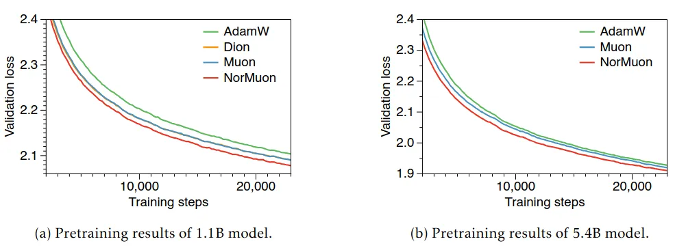
Empirically, NorMuon was shown to outperform both AdamW and Muon consistently across model scales. In a 1.1B parameter transformer pre-training, NorMuon achieved about 11% faster training (in terms of reaching a perplexity target) than Muon (and >21% faster than Adam). In a larger 5.4B parameter model, the gains were even higher (the draft reported up to 22% faster than Muon). NorMuon thus demonstrates that one can get much of the benefit of AdaMuon’s adaptivity with far less overhead, by focusing on the most significant normalization (per neuron) needed after orthogonalization. It underscores the idea that orthogonalization and adaptive rates are complementary: Muon fixes global conditioning, and a light-weight normalization fixes per-neuron imbalances, resulting in a highly efficient optimizer for very large networks.
Conclusion
From its inception in late 2024, Muon has grown from a clever idea on orthogonalizing momentum into a family of optimizers pushing the frontier of training efficiency. We saw how the original Muon introduced the concept of orthogonal updates that improve learning in under-represented directions. Theoretical work connected Muon to dual gradient descent under RMS norms, explaining its width-scalability. Subsequent adaptations tackled practical challenges: scaling to LLMs with weight decay and update rescaling, provable faster convergence under low-rank structure, and the incorporation of adaptive learning rates (AdaMuon and NorMuon) to further boost performance while keeping efficiency. These milestones are summarized in the table below:
| Milestone | Date | Key Contribution | Impact on Training |
|---|---|---|---|
| Original Muon | Oct 2024 | Orthogonalized momentum updates via Newton–Schulz | Set speed records (e.g. NanoGPT, CIFAR-10); improved sample efficiency |
| Scaling to LLMs (Moonshot) | Feb 2025 | Added weight decay and RMS-aligned update scaling | ~2× efficiency vs AdamW; Enabled 1.5B+ model training (Moonlight MoE); half memory via ZeRO-1 |
| Theoretical Derivation (Bernstein) | Mar 2025 | Derived Muon as steepest descent under RMS norm; width-independent learning rates | Provided modular DL framework and understanding of Muon’s advantages |
| Convergence Analysis | May 2025 | Proved faster rates for Muon under low-rank Hessians (non-convex and star-convex cases) | Theoretical validation of Muon’s efficiency when gradient subspace is limited (common in deep nets) |
| AdaMuon | Jul 2025 | Introduced element-wise adaptivity (variance correction) after orthogonalization; sign-stabilized updates | 40%+ training speedup over AdamW on large models; outperformed base Muon by 10–30% |
| NorMuon | Oct 2025 | Introduced neuron-wise normalized updates for efficiency; distributed-friendly implementation | Further 11–22% speedup over Muon in 1B–5B models; memory overhead on par with Muon, much lower than AdamW |
Throughout its evolution, Muon has exemplified how combining linear algebra insights with adaptive optimization can yield powerful new algorithms. As neural networks continue to grow in size and complexity, such optimizers that orthogonalize and normalize updates appear promising for the future of efficient AI training. Muon’s story, from a blog post to state-of-the-art results in one year, also highlights the rapid pace of innovation in optimization research, driven by both practical speedrunning and deep theoretical ideas. The journey of Muon is likely far from over, as researchers continue to refine these methods for even larger models and diverse architectures.
Experiments
This notebook here presents a benchmark evaluating three optimizers, AdamW, Muon, and AdaMuon, on a lightweight transformer model (~3.4M parameters). The goal was to empirically compare convergence dynamics, stability, and final performance when training a small-scale language model on the WikiText-2 dataset.
Setup
A character-level tokenizer (SimpleCharTokenizer) was built directly from the dataset vocabulary, avoiding subword segmentation to keep the training pipeline fully interpretable. The model input sequences were limited to 256 tokens, each embedded in a 256-dimensional latent space. The network consisted of 4 transformer blocks, each with 4 attention heads and 1,024 feed-forward units, followed by a final projection head for next-token prediction.
Training used mixed precision (AMP) and a cosine learning rate schedule with linear warm-up for the first 1,000 steps. Optimizers shared a weight decay of 0.1 but differed in their configuration:
- AdamW:
lr=1e-3(baseline optimizer) - Muon:
lr=3e-3,momentum=0.95,rms_target=0.1 - AdaMuon: same as Muon + adaptive second-moment normalization (, )
Each model was trained for 15 epochs, and validation loss was computed after each epoch.
Results
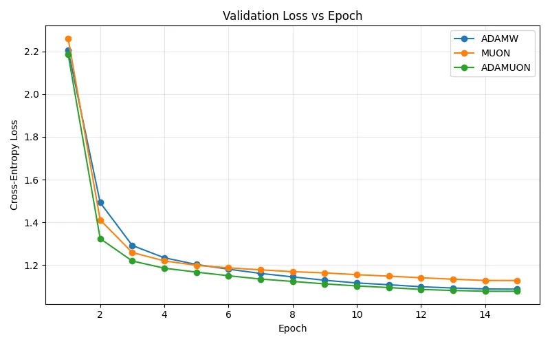
All models exhibited smooth convergence, but their behaviors diverged in subtle ways:
| Optimizer | Initial Loss | Final Loss | Convergence Behavior |
|---|---|---|---|
| AdamW | 2.21 | 1.087 | Fast early convergence, stable plateau |
| Muon | 2.26 | 1.127 | Slower descent, smoother gradients |
| AdaMuon | 2.19 | 1.077 | Fastest and most stable convergence |
The validation loss curves show that AdamW and Muon reach similar minima, while AdaMuon consistently performs better throughout training, combining the orthogonal stability of Muon with the adaptivity of Adam-like optimizers. Muon’s slightly slower convergence reflects its geometric regularization, which encourages orthogonalized, less redundant updates. In contrast, AdaMuon’s adaptive scaling allows it to balance global step uniformity with local variance correction, yielding the lowest final loss.
Conclusion
The experiment confirms that Muon and AdaMuon are viable alternatives to AdamW, maintaining comparable training efficiency while improving optimization geometry. In particular, AdaMuon achieved the best validation loss (1.077) and demonstrated more stable learning dynamics, validating its hybrid design.
These findings, though obtained on a small-scale GPT model, highlight how geometry-aware optimizers like Muon can enhance convergence behavior in language models, especially when extended with adaptive normalization mechanisms.